Hey everyone! You may have heard already about DynaMaps. It’s been out for about a month now. Reception has been overwhelmingly positive, thanks to all those who gave it a shot and sent their valuable feedback. A presentation was published on the Dynamo Blog for the first release, but it’s evolving so fast it seems usefull to present some of the possible workflows. So here we go!
As explained in the Dynamo Blog Post, DynaMaps is a package containing a ViewExtension as well as a set of nodes :
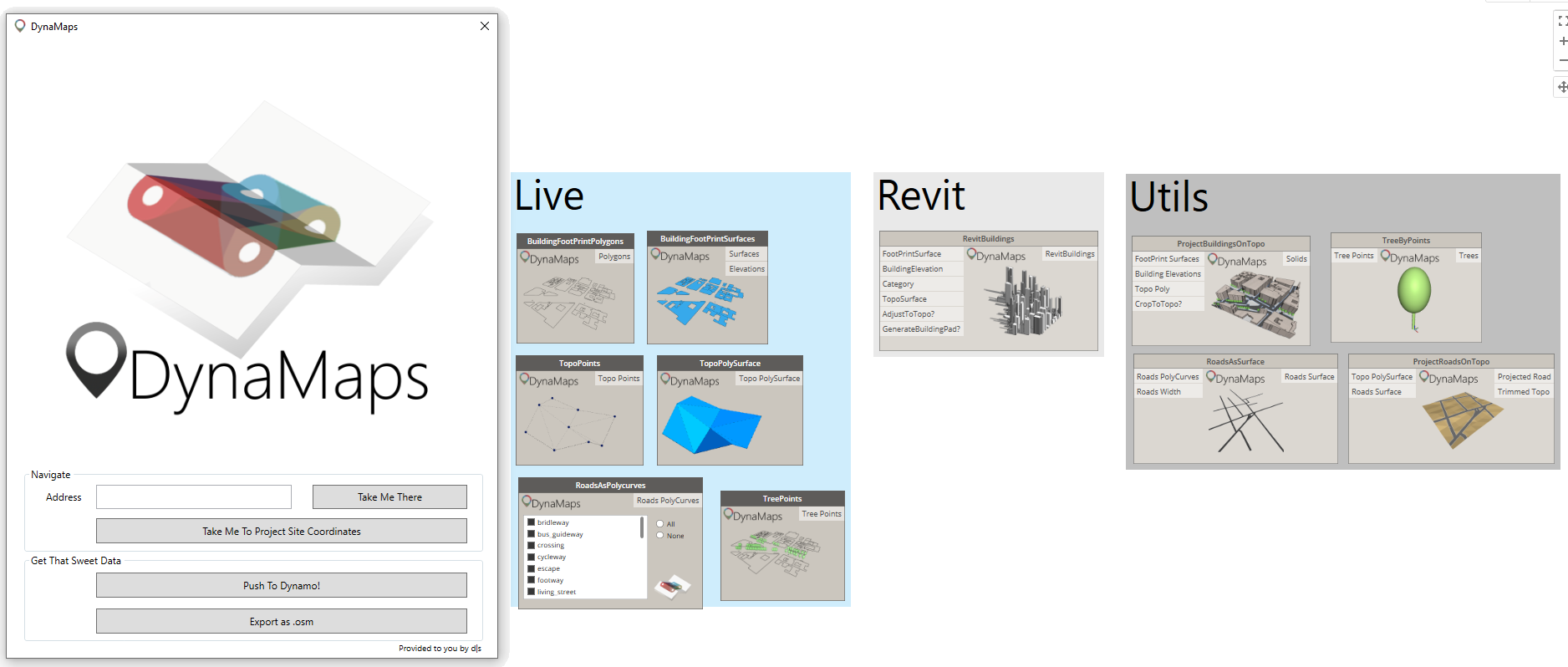
The nodes were made to import site geometry inside Dynamo in the most straightforward way. They are sorted in three categories:
- Live : Nodes that harness data from the selected area in the DynaMaps View Extension. They are the link between the view extension and the rest of your graph.
- Revit : Nodes that use DynaMaps Data to create Revit Geometry in a very straightforward way. So far there is only RevitBuildings but more are on their way!
- Utils : Those are made to ease some common operations on geometry. They all work from the DynaMaps Live nodes data.
Here’s a step by step demonstrations on how to get all site geometry inside dynamo. In a future blogpost, we’ll document a workflow to create Revit site geometry using DynaMaps.
GETTING ALL SITE GEOMETRY INSIDE DYNAMO
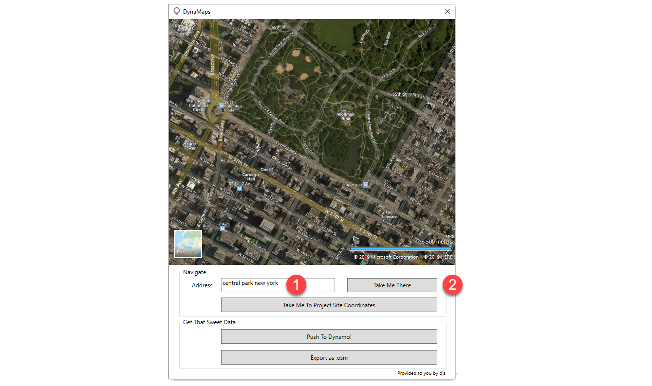
Step 1 : Selecting your site area
Open the DynaMaps view extension from the “View” tab of dynamo, enter your address (1) and press “Take Me There” (2). You can navigate the map just like in google maps, zoom in/zoom out and slide it. There’s even a satellite mode! 🙂
Note: if you have entered the latitude and longitude of your site, you may press “Take Me To Project Site Location”. That will automatically place the map on your project location point and all geometry will be brought in it’s correct location. The latitude and longitude need to be those of your project base point!
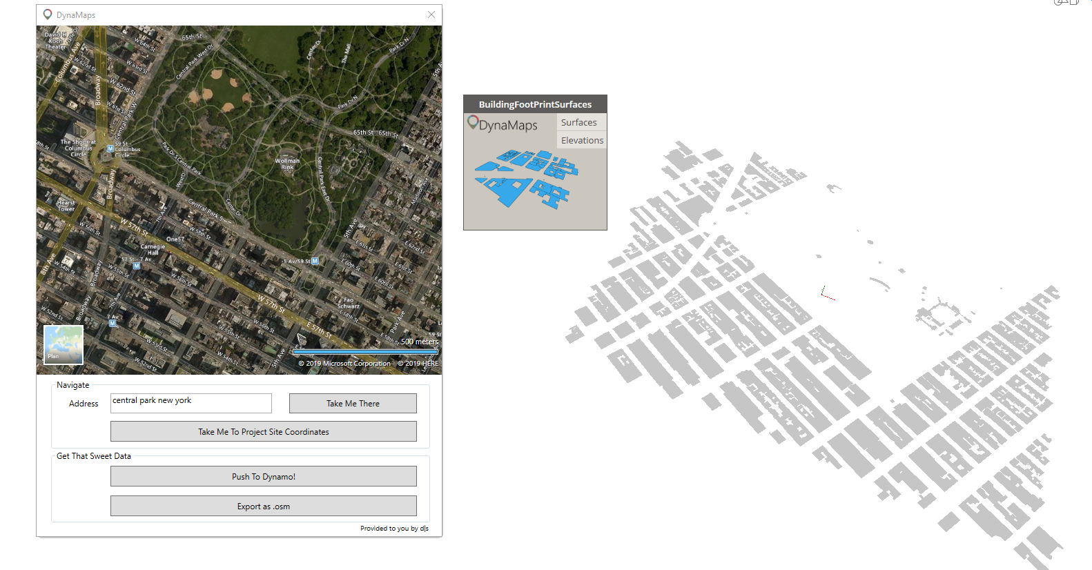
Step 2 : Pushing the data to dynamo
In this workflow, we’ll start by bringing the building footprints as surfaces. I order to do so, place the node on the canvass and press “Push To Dynamo” on the view extension. We recommand working in manual mode. If you didn’t get too crazy with the size of the area – which I kind of did here – it shouldn’t take too long for this to appear:
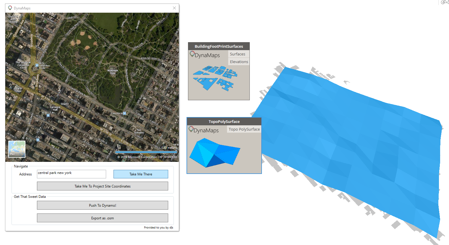
Step 3 : Getting the topography in Dynamo
Getting the topography in dynamo using DynaMaps is very direct. All you need to do is place a TopoAsPolySurface or TopoPoints (depending on what you wish to do) and hit “execute”. The data is from Nasa’s SRTM.
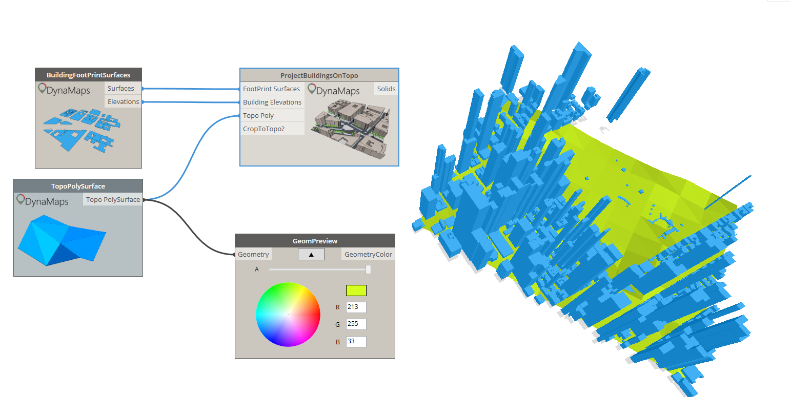
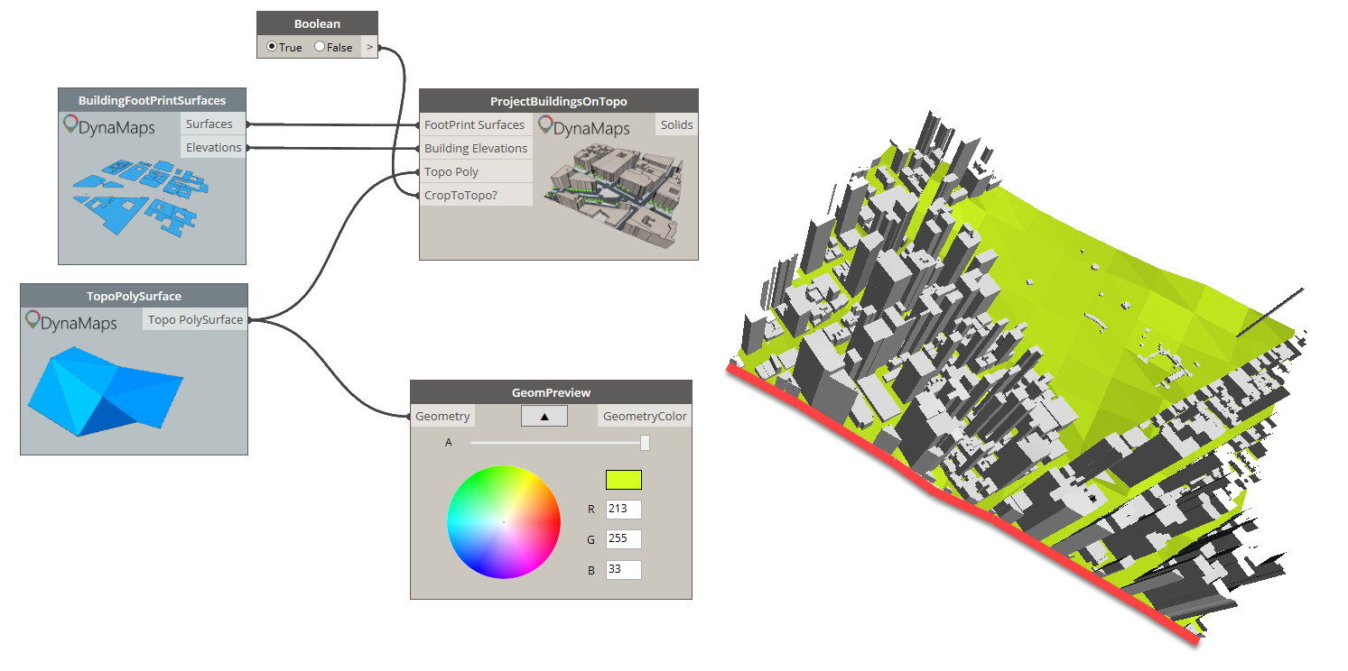
Step 4 : Creating the buildings 3D geometry
We will use another node from the DynaMaps Package to do so : “ProjectBuildingsOnTopo”. It will easilly create the 3D buildings and project them on the topography polysurface. The”CropToTopo” input is optional. When it is set to true, it allows to crop the the buildings in order to have a clean square of site geometry. The height of the buildings if from open street map (when it has been made available). If a building doesn’t have height information, a random value between the minimum and maximimum building heights of the area will be assigned. I’ve had a suggestion to make it possible to enter a default value for all buildings with no height data (thank you Mark Ackerley 🙂 !). It will be implemented in the next release.
Note : the GeomPreview node is only used for visualization purposes. It is from the Data Shapes Package. Also, from that point you can close the DynaMaps view extension to free up some screen space as you only need to push the data once into dynamo.
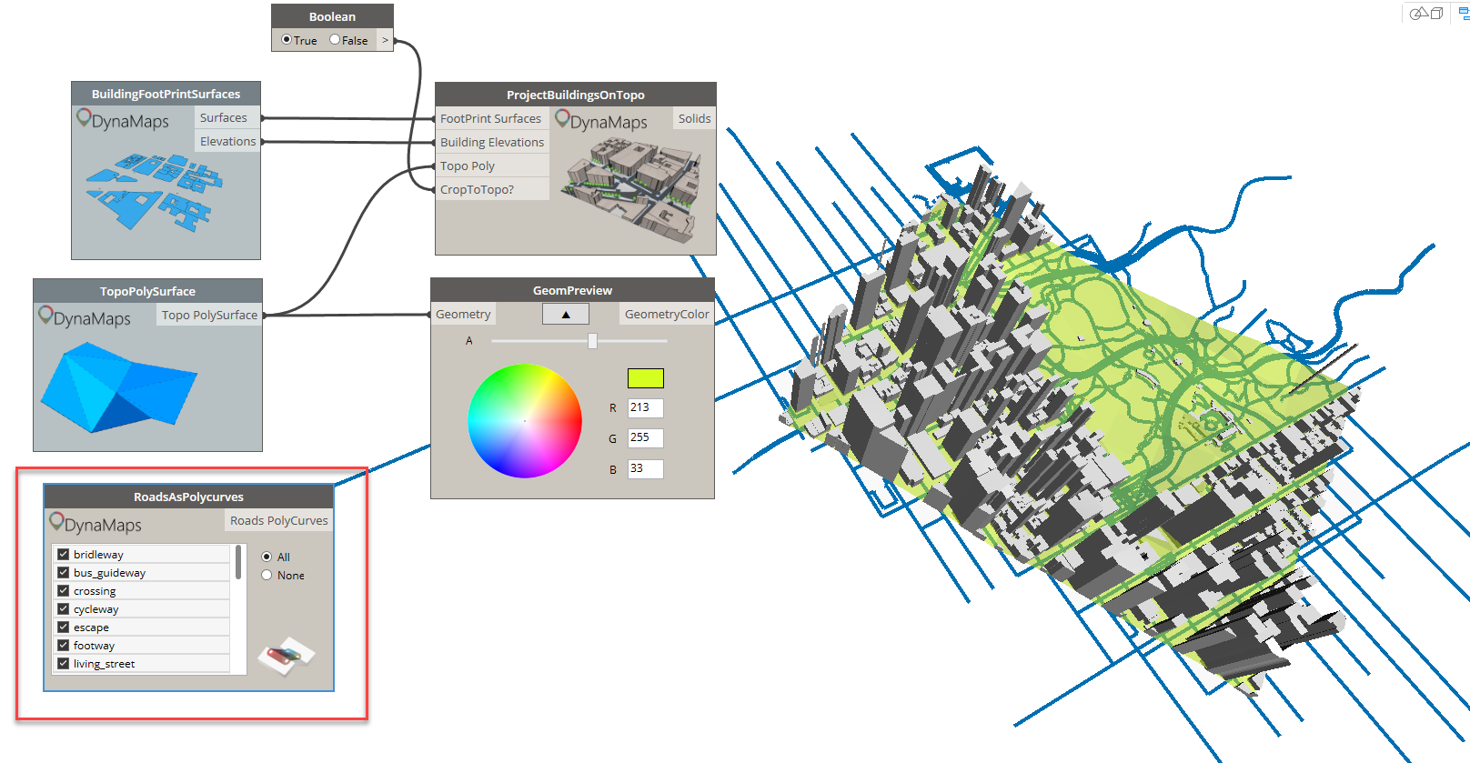
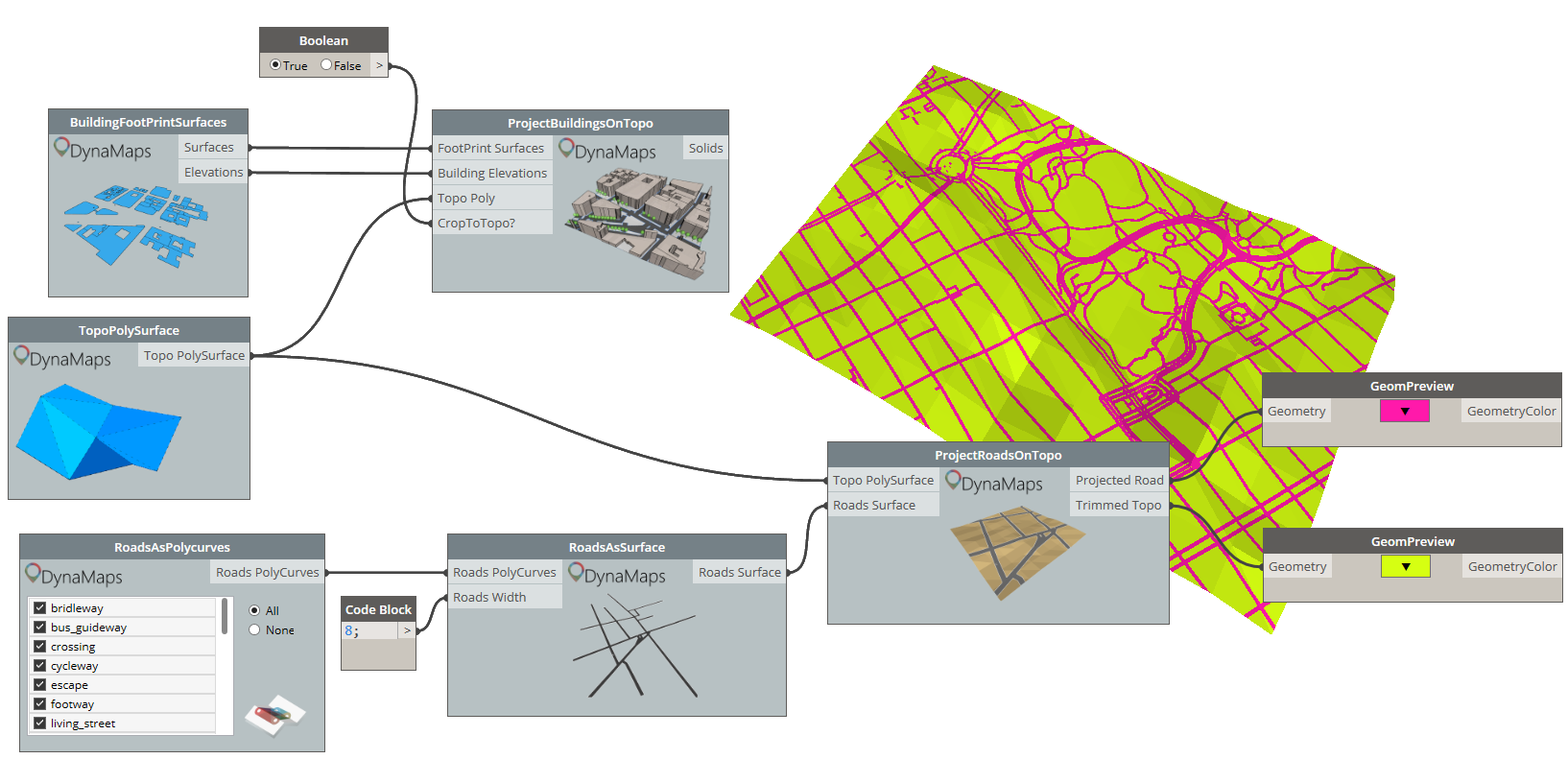
Step 5 : Getting the road geometry
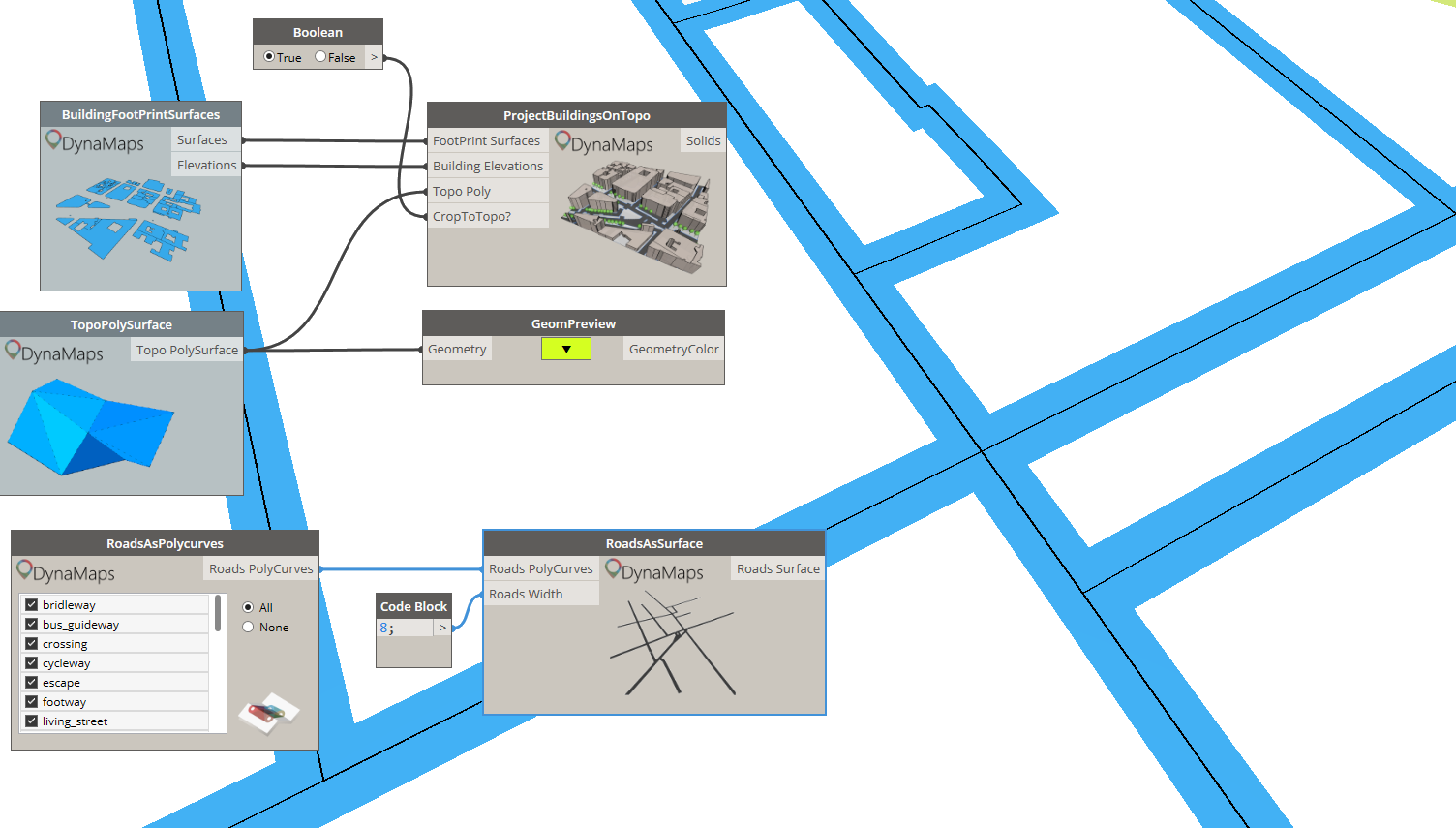
The starting point is the “RoasAsPolycurves” node from the Live category. It offers a list of all road types in open street map. You can select those you’re interested in and hit execute!
Those polycurves can be used to obtain surfaces, that can then be projected on the topo polysurface. The width of the roads has to be entered manually as there is very little useful data about it.
Projecting roads on the topography polysurface using the “ProjectRoadsOnTopo” node returns the projected roads as well as a trimmed topo polysurface. Those can be used and visualized separately.
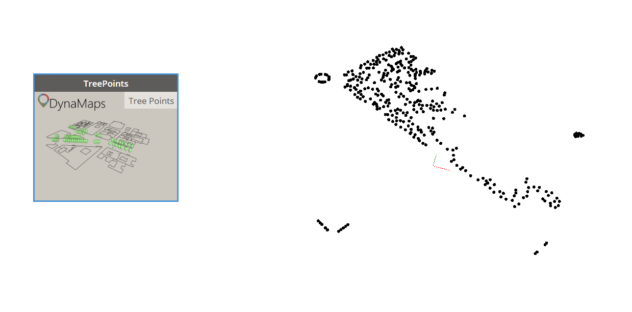
Step 6 : Trees!
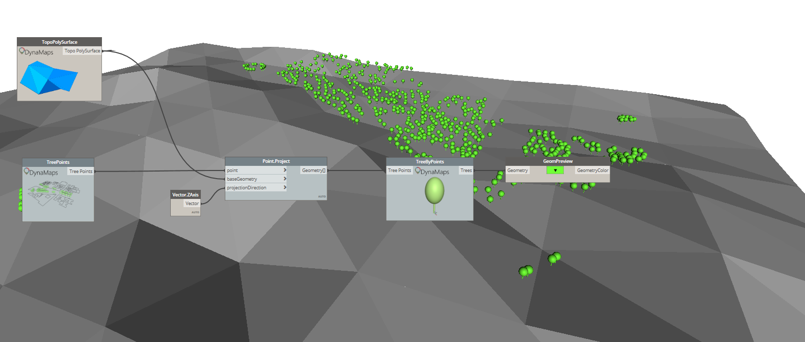
Once again, the starting point will be one of the Live nodes : “TreePoints”. It will output the location of all the trees of the selected area as points. Those can then be projected onto the topo polysurface.

And finally, just for the sake of having something aestetically pleasing, you can use the node “TreeByPoints” in order to have a little – very basic – tree geometry placed at each one of the projected points.
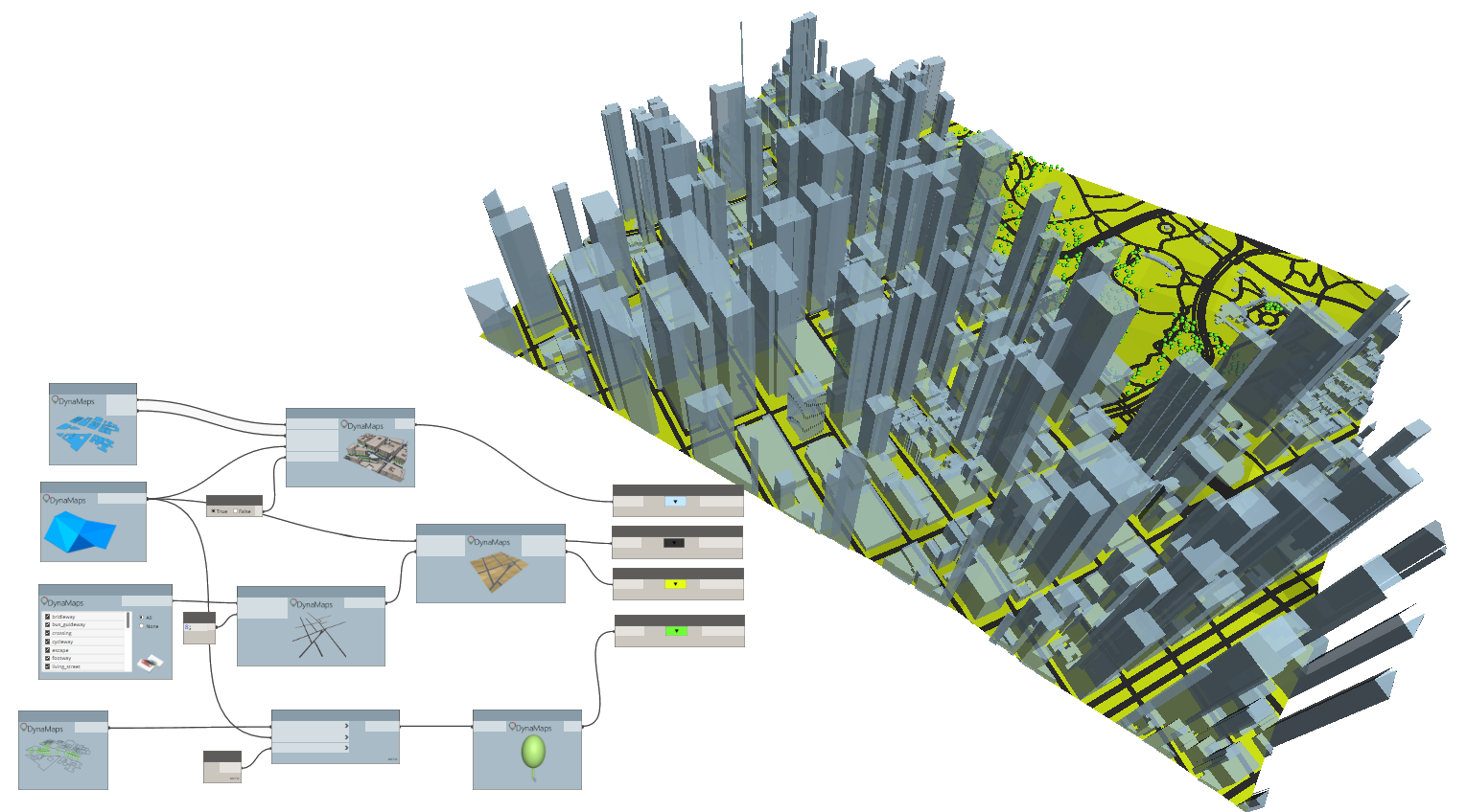
And that’s it! Here’s the general result :
Please feel free to comment on how you think this can be improved !


Leave a reply to Andrea Rolle Cancel reply